Bootstrap

Corresponding reading

• Chapter 4.6 in Agresti and Kateri (2021)
• Chapter 8.5, p 284 in Rice (2006)

The bootstrap is a resampling method for estimating measures of accuracy for the estimator (such as variance or confidence intervals) when obtaining them analytically is difficult. Resampling methods have become extremely common and absolutely indispensable in statistics due to the widespread availability of computing power. We use the bootstrap to quantify the uncertainty associated with an estimator.

We can view the sample as the population in two ways, leading to two different kinds of bootstrap.

1. We are willing to assume that the distribution of the population is from a particular parametric family of distributions. We estimate the parameters of that distribution, and then resample from the estimated distribution, using these samples to build a probability distribution for our parameter estimator. This method is called the parametric bootstrap. The results will be similar to what you would get if you manipulate the exact sampling distribution of your estimator under your distributional assumption.

2. We don’t know the population distribution, and don’t know if a parametric family is appropriate. We just resample from the sample. This is called a nonparametric bootstrap as we make no assumption about the distribution, and can be used in a very wide variety of situations. This makes no specific distributional assumptions about the data, so it is robust to parametric assumptions. But, as we will see, even the nonparametric bootstrap has assumptions, like assumptions of independence and sufficiently large sample size.

In what follows we are going to focus on the non-parametric bootstrap, since that is what is most commonly used in practice.

The basic idea of the bootstrap is to use the empirical distribution of the sample as an approximating distribution of the population when the sample is large. That is, we use the sample as a stand-in for the population, and resample from it.

The name comes from the phrase, “pull yourself up by your bootstraps” which means to succeed by your own cleverness/hard work - without getting help from others; here we estimating something tricky by cleverly reusing the same sample we started with.

Caution

Bootstrap works only if the sample is large enough to accurately represent the population distribution. Bootstrapping cannot fix the problem of using a small sample for inference.

We’re first going to go through the procedure before we try to understand why it works. The bootstrap procedure to approximate the sampling distribution for \(\hat\theta\), given a sample \(X_1, \ldots, X_n\) would be:

1. Compute the observed value of \(\hat\theta\) from our data
2. Let \(B\) be some large number (such as 5000).
3. For each \(b\), \(b = 1, 2, \ldots, B\), do the following steps:

1. Get a new sample of the same size, n by resampling with replacement from the original sample.
2. Compute the observed value of the estimator for this new sample, and call it \(\hat\theta_{(b)}^*\). Repeat steps (i) and (ii) to get \(\hat\theta_{(1)}^*, \hat\theta_{(2)}^*, \ldots, \hat\theta_{(B)}^*\). The \(*\) indicates that it is a bootstrap estimate, i.e. calculated from our bootstrap sample (the book doesn’t use the \(*\) in its notation, but it is a standard way to keep them separated from our \(\hat\theta\) estimated from our original data)

4. Estimate quantities from the distribution of \(\hat\theta_{(b)}^*\)

1. The mean of \(\hat\theta^*\) \[\overline{\theta^*}=\frac{1}{B}\sum_{i=1}^B\hat\theta_{(b)}^*\] can be used to estimate the bootstrap bias estimate, given by \[\widehat{bias}(\hat\theta)=\overline{\theta^*}-\hat\theta.\]
   

2. calculate the standard deviation of \(\hat\theta^*_i\) as \[\displaystyle \dfrac{1}{B-1} \sum_{i=1}^B \left(\hat\theta_i^*-\overline{\theta^*}\right)^2.\] This is the bootstrap estimate of the variance of \(\hat\theta\), and the square-root of this quantity gives us the bootstrap estimate of SE, denoted \(SE_{\mathrm{boot}}\).

3. Quantiles of the distribution of \(\hat\theta^*\), where \(q^*_{\alpha}\) is the \(\alpha\)th quantile of the bootstrap distribution, defined as \[q^*_{\alpha}: \frac{\{\# \hat\theta^* \le q^*_{\alpha}\}}{B}=\alpha\] i.e. the value such that the proportion of the data that is less than \(q^*_{\alpha}\) is equal to \(\alpha\). You can think of this like using the histogram as your data as your distribution and you want the area under your histogram to the left of \(q^*_{\alpha}\) to be equal to \(\alpha\).

We will use these quantiles to define confidence intervals, which we will get to in the next section.

Note

In fact, the above definition is not quite accurate -- because of the discreteness of your data you may not have a point $q^*_{\alpha}$ that gets you exactly $\alpha$. Actually there are a set of values that are valid quantiles for discrete distributions, and there are several standard choices for how to choose one (see `?quantile` in R). We are not going to worry about this too much, because $B$ is very large.

What is the bootstrap doing?

When we talk about confidence intervals that are based on the normal, or the \(t\)-distribution, we are relying on the asymptotic distribution of our estimator being approximately normal and/or distributional assumptions about our data to have the sampling distribution of our data.

Without those assumptions, in theory, to construct the sampling distribution of a sample statistic, we would have to draw all samples from the population, compute the statistic for each sample, and the distribution of these statistics is the sampling distribution.(Hesterberg 2015)

In practice, though, we have only one sample. This is where the bootstrap comes in. We draw samples from an estimate of the population distribution, and compute the statistic of interest for each sample.

The bootstrap is based on a principle we have encountered many times so far: if something is unknown, you substitute an estimate for it.

What do we use as an estimate for the population? Here is a nice diagram of the bootstrap, created by Deborah Nolan. You can view it in context in the notes for Stat 20:

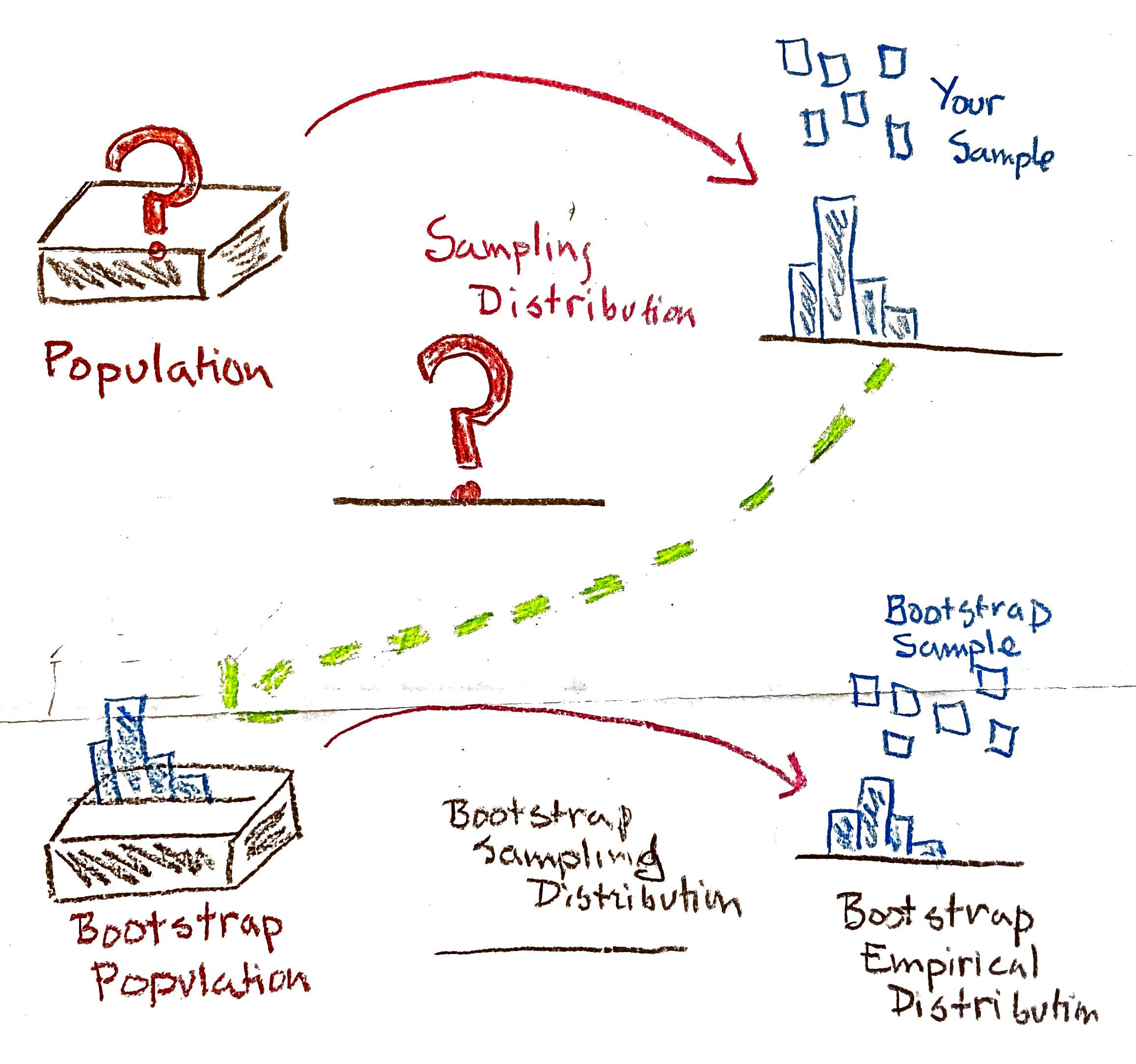
The most common method (which is the one we are covering) is the nonparametric bootstrap in which we draw samples with replacement from the sample. What we are actually doing is drawing samples from the empirical distribution \(\hat{F}_n\), defined by our sample \(X_1,\ldots,X_n\) which gives probability \(1/n\) to each observed observation in our sample, \[P(U=u) = \frac{1}{n}\sum_{i=1}^n I(X_i=u).\]

If we had infinite bootstrap samples the (\(B\rightarrow \infty\)) then \(\bar{\theta}^*\) and \(S_{boot}^2\) will converge to the mean and variance of the empirical CDF. Notice that this convergence is in \(B\), which we control and can make as big as we our computer can handle!

Note

In fact in principle, we could calculate the mean and variance of \(\hat\theta^*\) exactly, since we know the entire probability distribution of \(\hat{F}_n\) once we see our data, and the distribution of \(\hat\theta^*\) is just a function of a sample from \(\hat{F}_n\), but the computations would generally be too onerous.

An important point of difference between the sampling distribution of \(\hat\theta\) and the bootstrap distribution of \(\hat\theta^*\) is that the bootstrap distribution will be centered at the observed statistic, not the population parameter. This means we cannot generally use the bootstrap distribution to get a better estimate for the population parameter \(\theta\).¹ Instead, the bootstrap gives us an idea of the accuracy of the original estimate. Specifically, the quantity \(\hat\theta-\theta_0\) is well approximated by \(\hat\theta^*-\hat\theta\).

For example, for bias I want to estimate \[E(\hat\theta)-\theta_0,\] and so instead I use \[\frac{1}{B}\sum_{b=1}^B \hat\theta^*_{(b)}-\hat\theta\] Or for variance, I want to estimate \[E(\hat\theta-\theta_0)^2\] and instead I use \[ \frac{1}{B-1}\sum_{b=1}^B(\hat\theta^*_{(b)}-\hat\theta)^2\]

However, this means that we should be careful about using the quantiles of the bootstrap distribution of \(\hat\theta^*\) to estimate the quantiles of the sampling distribution of \(\hat\theta\) if our distribution is not symmetric. For this reason, there is a lot of attention in bootstrap as to how to best create confidence intervals.

Confidence intervals using the bootstrap

There are a number of ways to using the bootstrap to compute confidence intervals. Here are three ways of finding a \(100(1-\alpha)\%\) confidence interval (\(0<\alpha<1\)).

Bootstrap percentile interval

The confidence interval is given by \[(q^*_{\alpha/2}, q^*_{1-\alpha/2}),\] where \(q^*_{\alpha/2}\) is the \(\alpha/2\)th quantile of the bootstrap distribution and \(q^*_{1-\alpha/2}\) is the \((1-\alpha/2)\)th quantile of the bootstrap distribution.

Since (using our empirical distribution), \(P(\hat\theta^* \le q_{\alpha/2}) = \alpha/2\), and \(P(\hat\theta^* \le q_{1-\alpha/2}) = 1-\alpha/2\), the area captured in the middle is \(1-\alpha\), which is what we need.

Notice that the confidence intervals are not necessarily symmetric around \(\hat\theta\), depending on if the bootstrap distribution of \(\hat\theta^*\) is skewed.

This method seems intuitive – use the bootstrap distribution directly. However, this strategy seems to violate what we said before, namely that the bootstrap distribution of \(\hat\theta^*\) can’t be immediately substituted for the sampling distribution of \(\hat\theta\) and instead we should use \(\hat\theta^*-\hat\theta\) is a good estimate of \(\hat\theta-\theta_0\). However, the theoretical justification of the percentile method lies on more complex grounds; while the justification of the CI is beyond the scope of what we will cover, it is not based on the (incorrect) substitution of the bootstrap distribution for the sampling distribution.

The percentile method is far and away the most commonly used technique for building confidence intervals. It is usually fine if the sampling distribution of \(\hat\theta\) is not too skewed, which you can get a sense of by looking at the distribution of the \(\hat\theta^*\).

Bootstrap basic (pivotal) interval

This is sometimes called the reverse percentile interval and is the one defined in Rice (2006). It’s rationale looks more like our construction of normal CI and replaces \(\hat\theta-\theta_0\) in our probability computations with \(\hat\theta^*-\hat\theta\).

Define \(\delta = \hat\theta - \theta_0\), and suppose we know the distribution of \(\delta\). This means that we know the quantiles of this distribution, and if we want to capture the middle 95% of the values, we can use the 2.5th percentile and 97.5th percentiles to do this. Denote the 2.5th percentile by \(q_{0.025}\) and the 97.5th percentile by \(q_{0.975}\), \[P(\delta \le q_{0.025}) = 0.025 \quad P(\delta \le q_{0.975}) = 0.975\]

Then we have that: \[ P(q_{0.025}\le \delta \le q_{0.975}) = 0.95 \Rightarrow P(q_{0.025}\le \hat\theta - \theta_0 \le q_{0.975}) = 0.95 \] We can manipulate the inequalities to isolate \(\theta_0\) in the center, just like we did with normal intervals: \[ \begin{aligned} 0.95 &= P(q_{0.025}\le \hat\theta - \theta_0 \le q_{0.975})\\ &= P(q_{0.025} -\hat\theta \le - \theta_0 \le q_{0.975} -\hat\theta)\\ &= P(- q_{0.025} + \hat\theta \ge \theta_0 \ge - q_{0.975} + \hat\theta)\\ &= P( \hat\theta - q_{0.975}\le \theta_0 \le \hat\theta -q_{0.025}) \end{aligned} \] We could of course use any confidence level, \(1-\alpha\), \[ P( \hat\theta - q_{1-\alpha/2}\le \theta_0 \le \hat\theta -q_{\alpha/2}) = 1-\alpha. \] The only problem, of course, is that we don’t know the distribution of \(\delta = \hat\theta - \theta_0\), so we don’t know the quantiles \(q_{\alpha/2}\) and \(q_{1-\alpha/2}\). This is where we can use the bootstrap, to estimate \(q_{\alpha/2}\) and \(q_{1-\alpha/2}\). We will approximate the distribution of \(\hat\theta -\theta_0\) by the distribution of \(\delta^*=\hat\theta^* - \hat\theta\), giving us estimates \(\hat{q}_{\alpha/2},\hat{q}_{1-\alpha/2}\) and a CI \[(\hat\theta - \hat{q}_{1-\alpha/2}, \hat\theta - \hat{q}_{\alpha/2})\]

Relating Back to \(q^*_{\alpha}\)

Note that the quantiles of the approximated \(\delta\) distribution (using \(\delta^*=\hat\theta^* -\hat\theta\)) are just the quantiles of the \(\hat\theta^*\) distribution less \(\hat\theta\). That is, if we let \(\hat{q}_\alpha\) be the \(\alpha\)th quantile of the \(\delta^*\) distribution, and \(q_\alpha^*\) be the \(\alpha\)th quantile of the \(\hat\theta^*\) distribution, then \[\hat{q}_{\alpha} = q_\alpha^* - \hat\theta.\] Substituting this into our confidence interval above, we get that the basic \(100(1-\alpha)\%\) confidence interval for \(\theta_0\) can be written as \[(2\hat\theta - q_{1-\alpha/2}^*,2\hat\theta - q_{\alpha/2}^* ).\]

Notice that this is a “reverse” of use of the bootstrap quantiles from the percentile, which was: \[(q_{\alpha/2}, q_{1-\alpha/2}),\] If the sampling distribution of \(\hat\theta\) is symmetric, this will not matter, but if you have a skewed distribution, then these will give skewed CI intervals in opposite directions.

The normal or t interval

This is the simplest, and will be fine if the sampling distribution of \(\hat\theta\) is approximately normal. It is simply given by \(\hat\theta \pm z_{\alpha/2}\times SE_{\mathrm{boot}}\), where \(SE_{\mathrm{boot}}\) is the bootstrap estimate of the standard error of \(\theta\).

You can be more conservative in smaller samples and use \(t_{\alpha/2,n-1}\). This can be beneficial, because bootstrap CI in small samples tend to be narrower than they should be. You can think of the bootstrap distribution as suffering from the same bias problems as the MLE estimate of variance that uses \(\frac{1}{n}\) – the bootstrap underestimates the variability in smaller sample sizes. Using the \(t\) quantiles, which are larger, can help a bit, but ultimately the bootstrap is not a small-sample method.

Example of rainfall data (Rice 2006)

The data are from a study of the natural variability of rainfall. The rainfall of summer storms was measured by a network of rain gauges in southern Illinois for the years 1960–1964 (Rice 2006). The average amount of rainfall (in inches) from each storm, by year.

A snapshot of the data:

Rows: 227
Columns: 2
$ rain_inches <dbl> 0.020, 0.001, 0.001, 0.120, 0.080, 0.420, 1.720, 0.050, 0.…
$ year        <fct> 1960, 1960, 1960, 1960, 1960, 1960, 1960, 1960, 1960, 1960…

We can see that the data is quite skewed, with heavy right tails. Suppose we want to estimate the median \(\theta\) of the distribution of rainfall. The median will be more robust to large right tails. We’ve never discussed the sampling distribution of the median, and so we don’t immediately have any tools to make confidence intervals (in fact, the median is asymptotically normally distributed as well).

Let’s consider the nonparametric bootstrap. Our sample size is 227, so that will be the size of each sample we generate. We will set \(B = 10,000\). That means that we wil resample with replacement 10,000 times from the original sample. Each time, the size of the sample we draw will be 227, and we will compute the estimates \(\hat\theta*\).

Exercise/Question

What would happen if I didn’t sample with replacement?

In this next bit of code, we will first compute the 0.025th and 0.975th quantiles of the bootstrap distribution of the median

### Computing the lower and upper quantiles
med_lq_np <- quantile(boot_np, probs = 0.025, na.rm = TRUE)
med_uq_np <- quantile(boot_np, probs = 0.975, na.rm = TRUE)

Now we can create percentile confidence intervals:

## percentile confidence intervals
med_ci_np <- c(med_lq_np, med_uq_np)

cat("A percentile 95% CI for the median:\n ", med_ci_np)

A percentile 95% CI for the median:
  0.05 0.11

Notice that our estimate is

[1] 0.07

so our bootstrap confidence interval is not symmetric around our estimate.

We can compare to this to a pivotal or reverse percentile CI

## basic (pivotal) confidence intervals
med_ci_basic_np <- c(2*med_obs -med_uq_np, 2*med_obs -med_lq_np )
### 

cat("A 95% pivotal CI for the median:\n ", med_ci_basic_np)

A 95% pivotal CI for the median:
  0.03 0.09

Compare to asymptotic normal distribution

In fact, the distribution of the sample median from a population with a density function \(f(x)\) is asymptotically normal with mean that is \(\theta\), the true median of the \(f\) distribution, and variance \(\frac {1}{4nf(\theta)^{2}}\) and \[\hat\theta \sim N\left(\theta,\frac {1}{4nf(\theta)^{2}}\right)\] Notice how the asymptotics rely on the sampling distribution of the data. This isn’t different from our MLE, where \(I(\theta)\) depends on the distribution of our data.

Suppose we blindly assumed the data distribution was normal, this would give us \(f(\theta)=1/{\sqrt {2\pi \sigma ^{2}}}\) and \[\hat\theta\sim N(\theta, {\displaystyle ({\pi }/{2})\cdot (\sigma ^{2}/n)).}\] This would give us the following estimate of standard error of the median for this data (by plugging in \(S^2\) for \(\sigma^2\)):

asySe<-sd(il_rain$rain_inches)*sqrt(pi/2/length(il_rain$rain_inches))
asySe

[1] 0.03043098

Our bootstrap estimate of variance would be just calculating the standard deviation of our \(\hat\theta^2\),

sd(boot_np)

[1] 0.0144147

We see that our bootstrap asymptotic variance is much smaller.

Our asymptotic confidence interval based on normality would be

ci_norm<-c(median(il_rain$rain_inches)-qnorm(0.975)*asySe,median(il_rain$rain_inches)+qnorm(0.975)*asySe)
cat("Asy Normal CI:\n",ci_norm)

Asy Normal CI:
 0.01035638 0.1296436

References

Agresti, Alan, and Maria Kateri. 2021. Foundations of Statistics for Data Scientists. Chapman; Hall/CRC.

Hesterberg, Tim. 2015. “What Teachers Should Know about the Bootstrap: Resampling in the Undergraduate Statistics Curriculum.” The American Statistician 69 (4): 371–86. https://doi.org/10.1080/00031305.2015.1089789.

Rice, John A. 2006. Mathematical Statistics and Data Analysis. 3rd ed. Duxbury Press.

Footnotes

1. This is not 100% accurate. There is a technique in machine learning, called bagging, that uses the mean of the bootstrap distribution, \(\bar{\theta}^*\), as an improved estimator of \(\theta\) for the purpose of prediction in a regression context. This is only effective because of the kinds of estimators \(\hat\theta\) to which it is applied.